Does convexity suffice in Bohr–Mollerup?
The Bohr–Mollerup theorem characterizes the gamma function as the unique positive function on with , , and convex (log-convex). A natural question:
Question. If we keep and but weaken “log-convex” to merely convex, is still the unique solution?
Answer: no. Convexity is not enough. Since a positive log-convex function is automatically convex — and is convex increasing — replacing log-convexity by convexity is a strictly weaker hypothesis, so we should expect extra solutions, and indeed there are. This note exhibits an explicit one and proves it works.
1. Why the functional equation alone determines almost nothing¶
Fix any solution of and compare it with . Since as well, the ratio satisfies
So every solution has the form with an arbitrary 1-periodic positive function; normalization forces only . The solution set is therefore infinite-dimensional. A shape hypothesis is what collapses it: log-convexity forces (a convex periodic function is constant), giving . The question is whether plain convexity is a strong enough shape hypothesis. It is not.
Lean proof: ratio_periodic (every solution is times a 1-periodic function)
/-- **The solution space of the functional equation.** For *any* `F` obeying `F (y+1) = y F y`, the
ratio `F / Γ` is `1`-periodic; equivalently every solution equals `Γ` times a `1`-periodic function.
So positivity + functional equation + `F 1 = 1` leave an infinite-dimensional family of solutions,
and only a *shape* hypothesis (log-convexity, or — the question here — convexity) can hope to
single out `Γ`. -/
theorem ratio_periodic {F : ℝ → ℝ} (hF : ∀ y, 0 < y → F (y + 1) = y * F y)
    {x : ℝ} (hx : 0 < x) : F (x + 1) / Gamma (x + 1) = F x / Gamma x := by
  have hx' : x ≠ 0 := hx.ne'
  have hg : Gamma x ≠ 0 := (Gamma_pos_of_pos hx).ne'
  rw [hF x hx, Gamma_add_one hx.ne']
  field_simp
2. The counterexample¶
For a small parameter define the 1-periodic factor and the candidate function
Because , we have , and has period 1 with at every integer (as ). Hence, exactly as in §1:
Positivity: for .
Functional equation: .
Normalization: .
These three are elementary and fully machine-checked.
Lean: the periodic factor perturb (periodic, positive, at integers)
/-- The `1`-periodic factor `1 + ε (1 - cos 2πx)`. It is `≥ 1`, so positive for `ε ≥ 0`; it equals
`1` at every integer; and it has period `1`. Multiplying `Γ` by it therefore keeps positivity, the
functional equation `f (x+1) = x f x`, and the normalization `f 1 = 1`. -/
noncomputable def perturb (ε x : ℝ) : ℝ := 1 + ε * (1 - Real.cos (2 * π * x))

/-- `perturb` has period `1`, since `cos` has period `2π`. -/
theorem perturb_periodic (ε x : ℝ) : perturb ε (x + 1) = perturb ε x := by
  have h : Real.cos (2 * π * (x + 1)) = Real.cos (2 * π * x) := by
    rw [show 2 * π * (x + 1) = 2 * π * x + 2 * π by ring]; exact Real.cos_add_two_pi _
  unfold perturb; rw [h]

/-- `perturb` is positive for `ε ≥ 0`, because `1 - cos ≥ 0`. -/
theorem perturb_pos (hε : 0 ≤ ε) (x : ℝ) : 0 < perturb ε x := by
  have h : 0 ≤ ε * (1 - Real.cos (2 * π * x)) :=
    mul_nonneg hε (by linarith [Real.cos_le_one (2 * π * x)])
  unfold perturb; linarith

/-- `perturb ε 1 = 1`, since `cos 2π = 1`. -/
theorem perturb_one (ε : ℝ) : perturb ε 1 = 1 := by
  have h : Real.cos (2 * π * 1) = 1 := by
    rw [show 2 * π * 1 = 2 * π by ring]; exact Real.cos_two_pi
  unfold perturb; rw [h]; ring
Lean: f, its positivity f_pos, normalization f_one, and the functional equation f_functional_eq
/-- The counterexample candidate `fᵥ(x) = Γ(x) · (1 + ε (1 - cos 2πx))`. -/
noncomputable def f (ε x : ℝ) : ℝ := Gamma x * perturb ε x

/-- `fᵥ` is positive on `(0, ∞)` for `ε ≥ 0` (a product of positives). -/
theorem f_pos (hε : 0 ≤ ε) {x : ℝ} (hx : 0 < x) : 0 < f ε x :=
  mul_pos (Gamma_pos_of_pos hx) (perturb_pos hε x)

/-- **Normalization** `fᵥ 1 = 1`, from `Γ 1 = 1` and `perturb ε 1 = 1`. -/
theorem f_one (ε : ℝ) : f ε 1 = 1 := by
unfold f; rw [Gamma_one, perturb_one]; ring/-- **The Gamma functional equation is preserved**: `fᵥ (x + 1) = x · fᵥ x` for `x > 0`, because
`Γ (x+1) = x Γ x` and `perturb` has period `1`. -/
theorem f_functional_eq {x : ℝ} (hx : 0 < x) : f ε (x + 1) = x * f ε x := by
unfold f; rw [Gamma_add_one hx.ne', perturb_periodic]; ringThe convex counterexample is, to the eye, indistinguishable from :
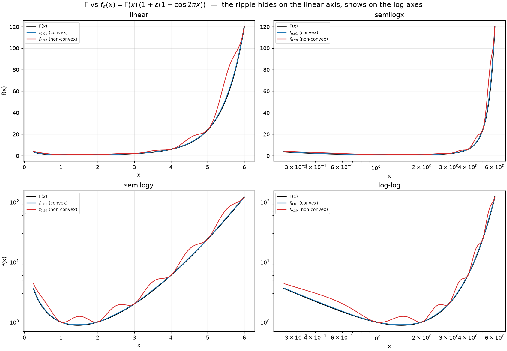
Figure 1: (black) and the convex counterexample (blue) coincide to the eye in all four scalings; a larger, non-convex (red) exposes the periodic ripple. The ripple is a few-percent relative modulation: swamped by factorial growth on the linear axes, but clearly visible on the logarithmic axes (bottom row), where multiplicative structure becomes additive.
3. It differs from , and it is not log-convex¶
At the half-integer, , so
hence whenever . Moreover is not
log-convex: if were convex on , then the log-convex
Bohr–Mollerup theorem (Mathlib’s Real.eq_Gamma_of_log_convex) — whose remaining hypotheses we
verified in §2 — would force , contradicting
(3). So sits strictly below log-convexity. Once we show in
§4 that it is nevertheless convex, the failure of the convex-hypothesis theorem is
complete.
Lean proof: f_half, f_ne_Gamma (), and not_logConvex
/-- The value at `x = 1/2`: `fᵥ(1/2) = Γ(1/2) · (1 + 2ε)`, since `cos π = -1`. -/
theorem f_half (ε : ℝ) : f ε (1 / 2) = Gamma (1 / 2) * (1 + 2 * ε) := by
  have hcos : Real.cos (2 * π * (1 / 2)) = -1 := by
    rw [show 2 * π * (1 / 2) = π by ring]; exact Real.cos_pi
  unfold f perturb; rw [hcos]; ring

/-- For `ε > 0`, `fᵥ` differs from `Γ`: they already disagree at `x = 1/2`, where
`fᵥ(1/2) = (1 + 2ε) Γ(1/2) > Γ(1/2)`. -/
theorem f_ne_Gamma (hε : 0 < ε) : ¬ Set.EqOn (f ε) Gamma (Ioi 0) := by
  intro hEq
  have h : f ε (1 / 2) = Gamma (1 / 2) := hEq (by norm_num : (1 / 2 : ℝ) ∈ Ioi (0 : ℝ))
  rw [f_half] at h
  have hg : 0 < Gamma (1 / 2 : ℝ) := Gamma_pos_of_pos (by norm_num)
nlinarith [h, mul_pos hg hε]/-- **`fᵥ` is not log-convex.** If `log ∘ fᵥ` were convex on `(0, ∞)`, then the log-convex
Bohr–Mollerup theorem `Real.eq_Gamma_of_log_convex` — whose other hypotheses (positivity, the
functional equation, `fᵥ 1 = 1`) we have verified — would force `fᵥ = Γ` on `(0, ∞)`, contradicting
`f_ne_Gamma`. So `fᵥ` lies strictly *below* log-convexity. Together with the convexity of `fᵥ`
(proved analytically in the note), this is exactly why convexity is too weak to characterize `Γ`. -/
theorem not_logConvex (hε : 0 < ε) : ¬ ConvexOn ℝ (Ioi 0) (log ∘ f ε) := by
intro hconv
have hEq : Set.EqOn (f ε) Gamma (Ioi 0) :=
Real.eq_Gamma_of_log_convex hconv (fun {_} hy => f_functional_eq hy)
(fun {_} hy => f_pos hε.le hy) (f_one ε)
exact f_ne_Gamma hε hEq4. It is convex (for small )¶
This is the crux. Write with . Since ,
Let (digamma) and (trigamma), so that and . We use two standard facts about :
because is positive and decreasing, and
Bounds on the perturbation. With we have and , and since ,
Both . Now split into two overlapping regions.
Region A: . Here (5) gives , so . Together with this yields .
Region B: , where is chosen (using (6)) so large that for all . Then , so , while (as ). Hence .
Coverage. As we have , so while pushes down to the unique zero of . Thus for all sufficiently small we have , the two regions cover , and everywhere. By (4), is convex.
For the concrete value the constants already close: , so , while is reached by already at . The next section confirms this numerically.
This entire argument is now machine-checked for . The linchpin is the trigamma lower bound, obtained from the trigamma recurrence (differentiate (6)), telescoping, and : since , letting gives .
Lean proof: trig_ge (the trigamma bound )
/-- **Trigamma lower bound** `(log Γ)''(x) ≥ 1/x` for `x > 0`. This is the one analytic fact the
note proves by hand; here it is machine-checked. From the digamma recurrence `ψ(x+1) = ψ(x) + 1/x`
we differentiate to get the trigamma recurrence `ψ'(x) = ψ'(x+1) + 1/x²`; telescoping and using
`ψ' ≥ 0` (convexity of `log Γ`) gives `ψ'(x) ≥ ∑_{k<n} 1/(x+k)² ≥ 1/x − 1/(x+n)`, and `n → ∞`
yields `ψ'(x) ≥ 1/x`. -/
theorem trig_ge {x : ℝ} (hx : 0 < x) : 1 / x ≤ trig x := by
  have key : ∀ n : ℕ, 1 / x - 1 / (x + n) ≤ trig x := by
    intro n
    have hsum_le : (∑ k ∈ Finset.range n, 1 / (x + (k:ℝ))^2) ≤ trig x := by
      rw [trig_telescope hx n]
      have : (0:ℝ) < x + n := by positivity
      linarith [trig_nonneg this]
    have hlb : 1 / x - 1 / (x + n) ≤ (∑ k ∈ Finset.range n, 1 / (x + (k:ℝ))^2) := by
      calc 1 / x - 1 / (x + n)
          = ∑ k ∈ Finset.range n, (1/(x+(k:ℝ)) - 1/(x+(k:ℝ)+1)) := (sum_tele n).symm
        _ ≤ ∑ k ∈ Finset.range n, 1 / (x + (k:ℝ))^2 := by
            apply Finset.sum_le_sum
            intro k _
            have hxk : (0:ℝ) < x + k := by positivity
            have hxk1 : (0:ℝ) < x + k + 1 := by positivity
            have e : 1/(x+(k:ℝ)) - 1/(x+(k:ℝ)+1) = 1/((x+k)*(x+k+1)) := by
              rw [div_sub_div _ _ (ne_of_gt hxk) (ne_of_gt hxk1), one_mul, mul_one]
              congr 1; ring
            rw [e]
            apply one_div_le_one_div_of_le (by positivity)
            nlinarith [hxk]
    linarith
  have hlim : Tendsto (fun n : ℕ => 1 / x - 1 / (x + n)) atTop (𝓝 (1 / x)) := by
    have hd : Tendsto (fun n : ℕ => x + (n:ℝ)) atTop atTop :=
      tendsto_atTop_add_const_left atTop x tendsto_natCast_atTop_atTop
    have h0 : Tendsto (fun n : ℕ => 1 / (x + (n:ℝ))) atTop (𝓝 0) :=
      (hd.inv_tendsto_atTop).congr (fun n => (one_div _).symm)
    simpa using (tendsto_const_nhds.sub h0)
  exact le_of_tendsto' hlim key
Lean proof: f_convex ( is convex on , via the two regions above)
/-- **The counterexample is convex** for `ε = 1/100`. Writing `f = exp u` with `u = log Γ + log g`,
convexity is `u'' + (u')² ≥ 0`. On `(0, 5/2]` the trigamma bound gives `u'' ≥ 1/x − C₂ ≥ 0`
(Region A); on `[5/2, ∞)` the digamma value `ψ(5/2) = 8/3 − γ − 2 log 2` and monotonicity give
`(u')² ≥ C₂ ≥ −u''` (Region B). Here `C₁ = 2πε`, `C₂ = 4π²ε(1+ε)`. -/
theorem f_convex : ConvexOn ℝ (Ioi 0) (f (1/100)) := by
  have hε : (0:ℝ) ≤ 1/100 := by norm_num
  refine convexOn_of_hasDerivWithinAt2_nonneg (convex_Ioi 0) ?_
    (f' := Fst (1/100)) (f'' := Snd (1/100)) ?_ ?_ ?_
  · exact fun x hx => (hasDerivAt_f hε hx).continuousAt.continuousWithinAt
  · intro x hx
    rw [interior_Ioi] at hx
    exact (hasDerivAt_f hε hx).hasDerivWithinAt
  · intro x hx
    rw [interior_Ioi] at hx
    exact (hasDerivAt_Fst hε hx).hasDerivWithinAt
  · intro x hx
    rw [interior_Ioi] at hx
    unfold Snd
exact mul_nonneg (f_pos hε hx).le (Q_nonneg hx)5. Numerical confirmation¶
Sampling on a fine grid over (second differences, step ) gives the minimum of :
| convex? | ||
|---|---|---|
| 0.010 | +0.48 | yes |
| 0.020 | +0.15 | yes |
| 0.025 | -0.013 | no |
| 0.030 | -0.21 | no |
| 0.040 | -0.74 | no |
So is convex for and loses convexity around — failing first in the tail, exactly where Region B is tightest. The headline value sits comfortably inside the convex range (). The trigamma bound (5), , was also checked pointwise and holds with room to spare.
6. Why log-convexity? Fitting exponential data without wiggles¶
Step back to what we are really doing: interpolating the factorials, i.e. fitting the points . These grow exponentially, so the natural canvas for them is the semilogy plot, where the points become . By Stirling, , so on that canvas they lie on a gently curving, almost straight line. A faithful interpolation should have no wiggles on either canvas — not on the ordinary linear plot, and not on this natural log plot.
These are two genuinely different requirements. The ripple is a relative (multiplicative) modulation of a few percent: against factorial growth it is invisible on the linear axis but plainly visible on the log axis, where multiplicative structure becomes additive (Figure 1). And the two “no wiggle” demands are exactly the two notions of convexity:
No wiggle on the linear plot convex monotone. This forbids the derivative from ever decreasing (the obvious S-shaped wiggle). It is necessary, but not sufficient: is convex yet still carries the ripple, because ’s curvature is strong enough to keep increasing while a small oscillation rides along.
No wiggle on the log plot log-convex monotone. The relative growth rate is the natural quantity for a multiplicatively-defined object — the functional equation multiplies by . Here fails: visibly turns over.
The two derivative tests side by side make this concrete: in the convex stays monotone (only the non-convex dips), whereas in the log-derivative the tiny ripple of is amplified to a clearly non-monotone wobble.
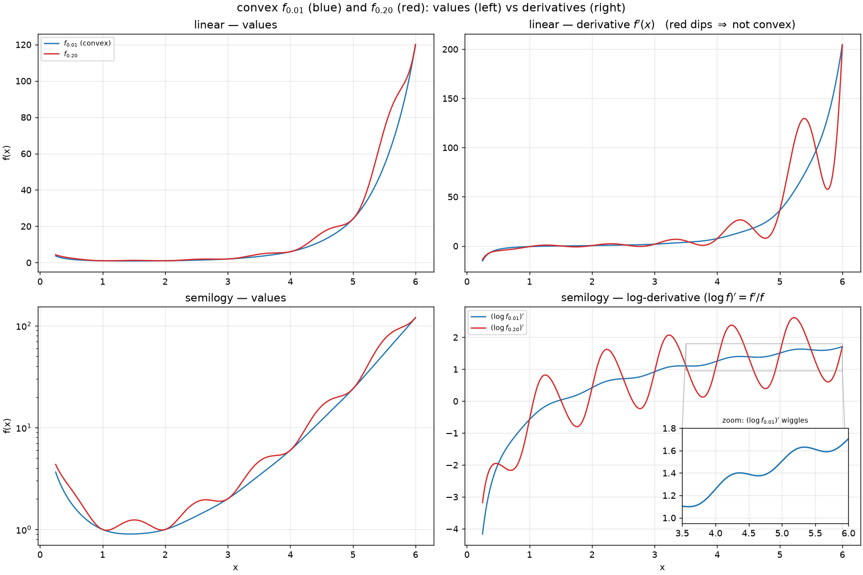
Figure 2:Values (left) versus derivatives (right) for (blue) and (red). The convex ripple is invisible in the values. In the ordinary derivative (top right) stays monotone — no wiggle, i.e. convex — while dips. In the log-derivative (bottom right, with zoom) visibly wiggles and turns over: it is not log-convex.
Because log-convex convex (for positive , since and is convex increasing), no wiggle on the log plot automatically implies no wiggle on the linear plot — it is the strictly stronger, and therefore decisive, requirement. That single demand — a smooth fit on the natural (log) canvas for exponential data — is exactly the log-convexity hypothesis, and by Bohr–Mollerup it pins down uniquely, whereas plain convexity does not.
7. What is proved where¶
Every hypothesis of the false theorem is machine-checked. For every , the bundled
statement convex_hypothesis_insufficient collects that is positive on ,
satisfies and , is not equal to ,
and is not log-convex.
Lean: convex_hypothesis_insufficient (positivity, functional equation, , not log-convex — for every )
/-- **Convexity is not sufficient (the machine-checked core).** For every `ε > 0`, `fᵥ` is a
positive solution of the Gamma functional equation with `fᵥ 1 = 1` that is **not** equal to `Γ` and
is **not** log-convex. The note proves analytically (and confirms numerically) that for small `ε`
(e.g. `ε = 1/100`) it is moreover **convex** — so, unlike log-convexity, plain convexity does not
determine `Γ`. -/
theorem convex_hypothesis_insufficient (hε : 0 < ε) :
    (∀ x, 0 < x → 0 < f ε x) ∧
      (∀ x, 0 < x → f ε (x + 1) = x * f ε x) ∧
      f ε 1 = 1 ∧
      ¬ Set.EqOn (f ε) Gamma (Ioi 0) ∧
      ¬ ConvexOn ℝ (Ioi 0) (log ∘ f ε) :=
  ⟨fun _ hx => f_pos hε.le hx, fun _ hx => f_functional_eq hx, f_one ε,
    f_ne_Gamma hε, not_logConvex hε⟩
The crux — that is also convex — is now machine-checked for the headline value
(f_convex, §4). Because current Mathlib has no di-/tri-gamma
theory, the Lean file builds it from scratch: it establishes the -smoothness of (from
the analyticity of the complex ), the digamma recurrence , and the
trigamma lower bound ; convexity then follows from the criterion, using
the digamma value (from Mathlib’s ) and monotonicity
of for the Region-B hand-off at . The single non-elementary numeric input is a
sharpened bound on the Euler–Mascheroni constant, obtained from Mathlib’s
and its precise bounds on .
The complete counterexample is bundled in convexity_hypotheses_hold: for ,
is positive, satisfies the functional equation and , is convex,
is not equal to , and is not log-convex — so convexity, normalization and the functional
equation together do not characterize .
Lean: convexity_hypotheses_hold (the full machine-checked counterexample at )
/-- **The counterexample satisfies every hypothesis of the (false) "convex Bohr–Mollerup"
theorem, yet is not `Γ`.** For `ε = 1/100`, `fᵥ` is positive on `(0, ∞)`, obeys the Gamma
functional equation `fᵥ(x+1) = x·fᵥ(x)`, is normalized `fᵥ 1 = 1`, is **convex** on `(0, ∞)`,
and is **not** log-convex — hence `fᵥ ≠ Γ`. So replacing "log-convex" by "convex" in
Bohr–Mollerup is false: convexity, normalization and the functional equation do **not** pin
down `Γ`. Every conjunct here is machine-checked (including the previously hand-proved
convexity). -/
theorem convexity_hypotheses_hold :
    (∀ x, 0 < x → 0 < f (1/100) x) ∧
      (∀ x, 0 < x → f (1/100) (x + 1) = x * f (1/100) x) ∧
      f (1/100) 1 = 1 ∧
      ConvexOn ℝ (Ioi 0) (f (1/100)) ∧
      ¬ Set.EqOn (f (1/100)) Gamma (Ioi 0) ∧
      ¬ ConvexOn ℝ (Ioi 0) (log ∘ f (1/100)) :=
  ⟨fun _ hx => f_pos (by norm_num) hx, fun _ hx => f_functional_eq hx, f_one _,
f_convex, f_ne_Gamma (by norm_num), not_logConvex (by norm_num)⟩Conclusion¶
Convexity does not replace log-convexity in the Bohr–Mollerup theorem: for every small the function is a convex, positive solution of with that is different from . The log-convexity hypothesis of the original theorem is therefore essential — it is exactly strong enough to eliminate the periodic perturbations that plain convexity tolerates. For this is now verified end-to-end in Lean, convexity included.
References¶
The companion note The Bohr–Mollerup theorem proves the log-convex version.
E. Artin, The Gamma Function Artin, 1964, discusses the role of log-convexity.
Bohr–Mollerup theorem on Wikipedia Wikipedia, 2025.
- Artin, E. (1964). The Gamma Function (M. Butler, Trans.). Holt, Rinehart.
- Wikipedia. (2025). Bohr–Mollerup theorem. https://en.wikipedia.org/wiki/Bohr%5C%25E2%5C%2580%5C%2593Mollerup_theorem