SO(3) Gauge Theory for Classical Mechanics
Abstract
We analyze the classical mechanics of the inverted spherical pendulum (ISP) and of the symmetrical (Lagrange) top as gauge theories in , the Lie group of rotations in three dimensions. We show that the equations of motion can be derived as geodesic equations on a curved manifold, , fibred over ordinary spacetime. This derivation is short and direct, standing in contrast to the more standard and elaborate delivery.
Adding a third angle , representing twist about the baton axis, introduces gyroscopic coupling that physically stabilizes the pendulum and converts the problem into that of the symmetrical top.
This formulation directly mirrors Yang-Mills theory and general relativity, showing that classical Newtonian mechanics can be elegantly expressed in terms of differential geometry.
The original version of this article in Wolfram Mathematica is published in Beckman, 2026.
Introduction
Gauge theory and gauge-covariant derivatives are the mathematical backbone of the Standard Model of particle physics, describing electromagnetic, weak, and strong interactions as connections on principal fibre bundles. Covariant derivatives on spacetime itself are the mathematical backbone of general relativity and gravitation. It is a seldom-mentioned, yet remarkable fact that exactly the same mathematical machinery pertains to classical Newtonian mechanics!
The unifying fact, promoted to a slogan, is:
“Forces arise as connection coefficients in covariant derivatives.”
Standard physics curricula derive the equations of motion for rotating rigid bodies using coordinate-heavy Euler-Lagrange equations written in Euler angles (yaw, pitch, and roll). This traditional approach—found in classic textbooks such as Goldstein’s Classical Mechanics Goldstein et al., 2002, Landau and Lifshitz’s Mechanics Landau & Lifshitz, 1976, or Arnol’d’s Mathematical Methods of Classical Mechanics Arnol'd, 2013—tends to obscure the overarching geometric structure.
In this article, we reformulate the classical inverted spherical pendulum (ISP) and Lagrange top geometrically, revealing the equations of motion following from a gauge-covariant absolute derivative along the system’s trajectory:
where is the absolute covariant derivative and the ’s are the connection coefficients of the specific gauge manifold we choose. In this article, the gauge manifold / gauge group is . In a future note, we will choose , specifically to avoid gimbal lock.
This is exactly the same kind of computation performed under the banner of gauge invariance in the Standard Model. Rather than postulating Coriolis or gyroscopic forces ad-hoc, they emerge naturally as the Christoffel connection coefficients of a curved manifold ( or ) fibred over ordinary time. Inertial forces arise from connection coefficients.
This formulation directly mirrors:
General Relativity: Where the gravitational force is replaced entirely by geodesic motion (vanishing covariant acceleration) in a curved 4D spacetime manifold.
Yang-Mills Gauge Theory: Where the gyroscopic off-diagonal coupling terms act exactly as a gauge potential , and the resulting Coriolis and gyroscopic precession forces emerge directly from the gauge-covariant derivative.
It is a remarkable fact that physics of all kinds—classical and quantum, relativistic and Newtonian—are concisely and elegantly unified through differential geometry. This note aims to furnish a concise, accessible bridge for physics undergraduates to see how gauge theory operates even in a simple, concrete classical system.
We accompany this note with:
A formal verification in Lean 4 verifying the algebraic properties of the 2D quotient metric and its singularity.
A symbolic verification in SymPy computing the Christoffel symbols, geodesic equations, and their limit, whereby the Lagrange top converges to the inverted spherical pendulum.
1. Lagrangian Formulation & Singularity
This section furnishes a “ground-truth” via the conventional and traditional derivation---Euler-Lagrange equations. Later, we show that the new, geodesical derivation yields exactly the same equations of motion.
Consider a rigid-rod pendulum of uniform density with mass and length , with its center of mass located at distance from the pivot, fixed to the 2D floor. We measure its angular position with two coordinates:
(pitch), measuring co-latitude from the North pole.
(cone-roll), measuring rotation around the original -axis.
The position of the center of mass in Cartesian coordinates is:
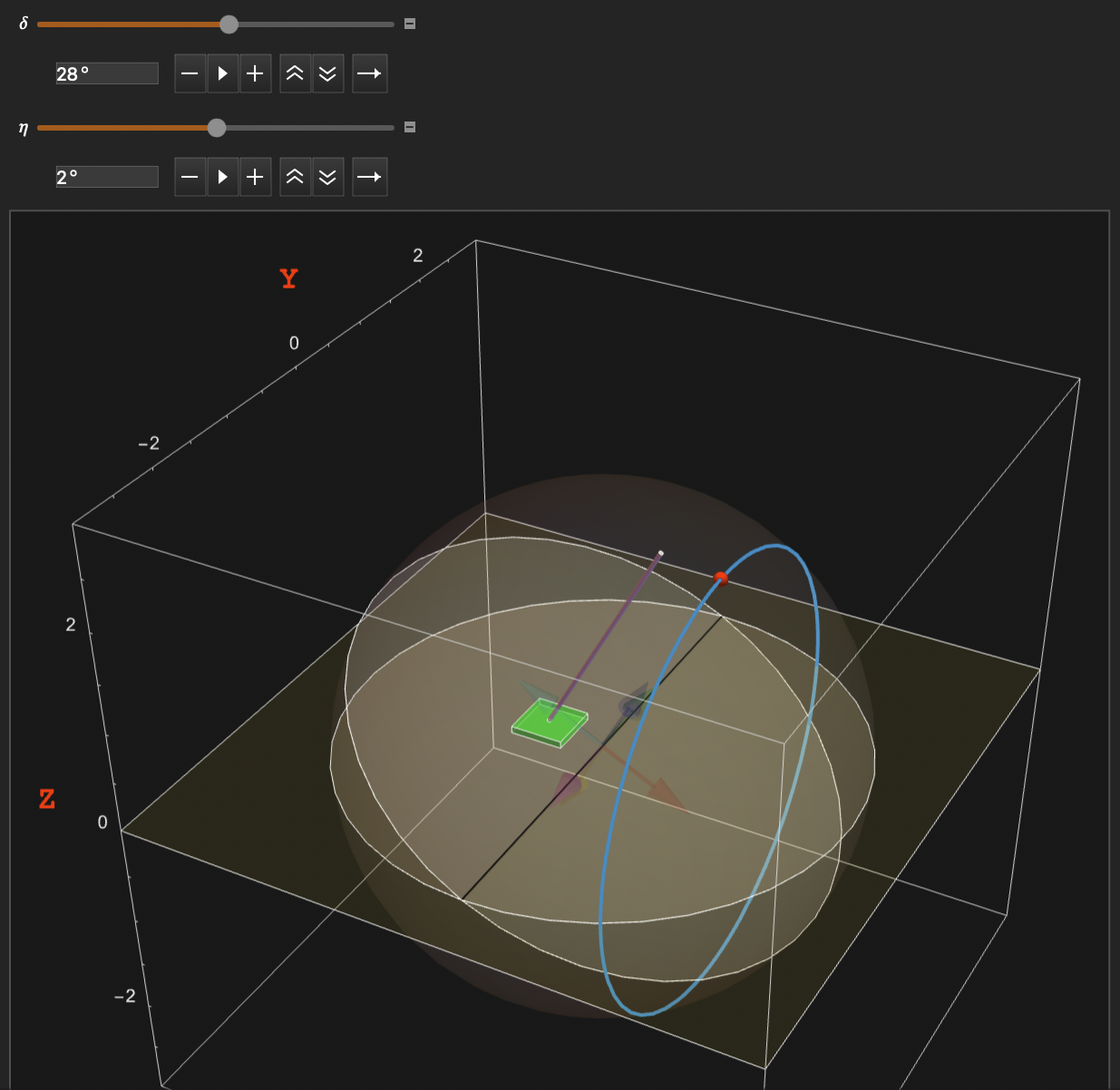
Figure 1:3D visualization of the inverted spherical pendulum showing the pitch () and cone-roll () coordinate system.
The velocity is , leading to the kinetic energy:
The potential energy under gravity pointing in the direction is:
With the Lagrangian , the Euler-Lagrange equations yield:
The Coordinate Singularity
The equation for contains the term , which diverges at the equator () for almost all values of . This is the mathematical manifestation of gimbal lock.
We can analyze the limits of the applied, gravitational, non-inertial force term in the direction, at the equator:
Typical Points (): If the pendulum is tilted away from the - plane (), the force term diverges:
This drives infinite azimuthal acceleration .
Exceptional Points (): If the pendulum swings purely within the - plane, then exactly. In this case, we have:
The force remains finite (and vanishes) at the equator because the gravity vector has no projection along the direction of azimuthal change. These trajectories can pass through the equator smoothly.
Indeterminate Limits: For general paths where , the limit is an indeterminate form and is path-dependent, reflecting the topological fact that the coordinate direction is undefined at the poles of the rotated coordinate system.
This gimbal-lock problem will be fully resolved in an upcoming note by performing the entire geometric computation again in , the double-cover rotation group that is free of coordinate singularities. A side-by-side video demonstration showing gimbal-lock divergence vs singularity-free stability is available in Beckman, 2026. A second video showing the mathematical equivalence of and trajectories away from the gimbal lock equator is available in Beckman, 2026. We thank the Wolfram Community for hosting these video attachments.
We formally define this metric and verify the vanishing of its determinant at the singularity in Lean 4:
Lean definition: metricSO3
/-- The 2D quotient metric tensor `g_μν` for the inverted spherical pendulum
in SO(3)/SO(2), represented as a diagonal matrix in pitch (δ) and cone-roll (η) coordinates. -/
def metricSO3 (I1 δ : ℝ) : Matrix (Fin 2) (Fin 2) ℝ :=
  !![I1, 0;
     0, I1 * (Real.cos δ) ^ 2]
Lean proof: det_metricSO3
/-- The determinant of the 2D metric tensor is `I1^2 * cos^2(δ)`.
This determinant vanishes at `δ = ±π/2` (90 degrees), causing the coordinate singularity. -/
theorem det_metricSO3 (I1 δ : ℝ) :
    (metricSO3 I1 δ).det = I1 ^ 2 * (Real.cos δ) ^ 2 := by
  unfold metricSO3
  rw [Matrix.det_fin_two_of]
  ring
2. Geometric Derivation via Kinetic-Energy Metric
Instead of the Euler-Lagrange formalism, we can derive the exact same equations of motion geometrically. The kinetic energy defines a Riemannian metric tensor on the 2D configuration space:
where . The inverse (contravariant) metric is:
which we formally define in Lean 4 as:
Lean definition: invMetricSO3
/-- The inverse metric tensor `g^μν` for the inverted spherical pendulum. -/
def invMetricSO3 (I1 δ : ℝ) : Matrix (Fin 2) (Fin 2) ℝ :=
  !![1 / I1, 0;
     0, 1 / (I1 * (Real.cos δ) ^ 2)]
We prove in Lean that the inverse is valid as long as we are away from the singularity:
Lean proof: metricSO3_mul_inv
/-- Verifies that `invMetricSO3` is indeed the matrix inverse of `metricSO3`
when `I1` is non-zero and the pendulum is not at the coordinate singularity (`cos δ ≠ 0`). -/
theorem metricSO3_mul_inv (I1 δ : ℝ) (hI1 : I1 ≠ 0) (hcos : Real.cos δ ≠ 0) :
    metricSO3 I1 δ * invMetricSO3 I1 δ = 1 := by
  unfold metricSO3 invMetricSO3
  ext i j
  fin_cases i <;> fin_cases j
  · simp [Matrix.mul_apply]
    field_simp [hI1]
  · simp [Matrix.mul_apply]
  · simp [Matrix.mul_apply]
  · simp [Matrix.mul_apply]
    have h_mul : I1 * Real.cos δ ^ 2 ≠ 0 := mul_ne_zero hI1 (pow_ne_zero 2 hcos)
    field_simp [h_mul]
The Christoffel symbols of the second kind are computed from the metric via:
The non-vanishing independent Christoffel symbols are:
Centrifugal and Coriolis Forces from Connection Coefficients
By expanding the geodesic equation for each coordinate, we can identify these connection coefficients with familiar physical forces.
For the pitch coordinate :
Here, the inertial term is proportional to the square of the velocity . This is the centrifugal force acting on the pitch angle due to the azimuthal roll of the pendulum.
For the roll coordinate :
Here, the inertial term is proportional to the product of two distinct velocities . This is the Coriolis force, arising from the interaction of radial (pitch) and azimuthal (roll) motions.
This is the precise realization of the governing slogan at the top of this note:
“Forces arise as connection coefficients in covariant derivatives.”
In standard Newtonian mechanics, these inertial forces are introduced ad-hoc as “fictitious” corrections for working in a rotating reference frame. Here, they are not postulated at all; they are the geometric consequence of the connection coefficients in the absolute covariant derivative along the curved trajectory.
The geodesic equation of motion incorporating the potential gradient force is:
where the force vector .
Let’s grind through this computation explicitly. First, we compute the coordinate derivatives of the potential energy :
Using the inverse metric where , we obtain the contravariant force components:
Substituting these force components and the non-vanishing Christoffel symbols back into the geodesic equations:
For :
Solving for yields:
which matches the Euler-Lagrange equation for character-for-character.
For :
Solving for yields:
which matches the Euler-Lagrange equation for character-for-character.
3. Gyroscopic Fibration via 
To include gyroscopic effects, we add a third angle , representing twist or spin around the long axis of the baton. The configuration space is now the full Lie group , viewed as a circle bundle (fibration) over the sphere.
Let be the moment of inertia around the spin axis, and be the transverse moment of inertia. The 3D metric tensor is:
Its inverse (contravariant) metric tensor is:
The off-diagonal elements of the metric tensor represent the gauge potential. As the baton moves along the cone-roll coordinate , the motion leaks into the twist coordinate via the gauge connection, physically manifesting as Coriolis and gyroscopic precession forces.
The resulting equations of motion are:
When , the first two equations devolve exactly to the 2D quotient equations of motion.
4. SymPy Symbolic Verification
We implement the metrics, Christoffel symbol computations, and covariant derivative equations of motion in Python using SymPy. The script verifies all algebraic steps and confirms the correctness of the limit against the 2D Euler-Lagrange equations.
import sympy as sp

# 1. Define symbolic variables
delta, eta, psi = sp.symbols('delta eta psi', real=True)
d_delta, d_eta, d_psi = sp.symbols('d_delta d_eta d_psi', real=True)
dd_delta, dd_eta, dd_psi = sp.symbols('dd_delta dd_eta dd_psi', real=True)

I1, I3, m, cz, g = sp.symbols('I1 I3 m cz g', positive=True)

coords = [delta, eta, psi]
vels = [d_delta, d_eta, d_psi]
accels = [dd_delta, dd_eta, dd_psi]

# 2. Define the metric tensor g_μν (metric3)
# Row 0: delta
# Row 1: eta
# Row 2: psi
metric = sp.Matrix([
    [I1, 0, 0],
    [0, I1 * sp.cos(delta)**2 + I3 * sp.sin(delta)**2, I3 * sp.sin(delta)],
    [0, I3 * sp.sin(delta), I3]
])

print("--- Metric Tensor g_μν ---")
sp.pprint(metric)

# 3. Compute the inverse metric g^μν
inv_metric = sp.simplify(metric.inv())
print("\n--- Inverse Metric Tensor g^μν ---")
sp.pprint(inv_metric)

# 4. Compute Christoffel symbols of the first kind:
# Γ_αβγ = 0.5 * (dg_{βγ}/dx^α + dg_{αγ}/dx^β - dg_{αβ}/dx^γ)
# Note: we use indices 0, 1, 2 corresponding to delta, eta, psi.
def get_g_first(a, b, c):
    # partial derivatives
    term1 = sp.diff(metric[b, c], coords[a])
    term2 = sp.diff(metric[a, c], coords[b])
    term3 = sp.diff(metric[a, b], coords[c])
    return sp.simplify(0.5 * (term1 + term2 - term3))

# Compute Christoffel symbols of the second kind:
# Γ^μ_αβ = g^μγ * Γ_αβγ
def get_christoffel(mu, a, b):
    val = 0
    for gamma in range(3):
        val += inv_metric[mu, gamma] * get_g_first(a, b, gamma)
    return sp.simplify(val)

# 5. Compute geodesic acceleration term: sum_{a,b} Γ^mu_ab * dot{x}^a * dot{x}^b
geodesic_terms = []
for mu in range(3):
    term = 0
    for a in range(3):
        for b in range(3):
            term += get_christoffel(mu, a, b) * vels[a] * vels[b]
    geodesic_terms.append(sp.simplify(term))

# 6. Define the Potential Energy and compute Potential Forces
# V = m * g * cz * cos(delta) * cos(eta)
V = m * g * cz * sp.cos(delta) * sp.cos(eta)
print(f"\nPotential Energy V: {V}")

# F^μ = -g^μν * dV/dx^ν
dV = sp.Matrix([sp.diff(V, c) for c in coords])
potential_forces = sp.simplify(-inv_metric * dV)

# 7. Equations of motion: ddot{x}^μ + geodesic_term = F^μ
eom = []
for mu in range(3):
    lhs = accels[mu] + geodesic_terms[mu]
    rhs = potential_forces[mu]
    eom.append(sp.Eq(lhs, rhs))

print("\n--- Equations of Motion (3D Gyroscope) ---")
for idx, coord in enumerate(coords):
    print(f"\nCoordinate: {coord}")
    sp.pprint(eom[idx])

# 8. Devolve to 2D case by setting I3 -> 0, I1 -> cz^2, m -> 1
print("\n--- Devolved Equations of Motion (I3 -> 0, I1 -> cz^2, m -> 1) ---")
devol_subs = {I3: 0, I1: cz**2, m: 1}
devol_eom = []
for mu in range(2): # only delta and eta
    # solve the equations for accelerations dd_delta and dd_eta
    eq = eom[mu].subs(devol_subs)
    acc = accels[mu]
    sol = sp.solve(eq, acc)[0]
    devol_eom.append(sp.Eq(acc, sp.simplify(sol)))

for idx, coord in enumerate(coords[:2]):
    print(f"\nDevolved Coordinate: {coord}")
    sp.pprint(devol_eom[idx])

# 9. Verify against 2D Euler-Lagrange equations
# dd_delta == sin(delta) * (g/cz * cos(eta) - cos(delta) * d_eta**2)
# dd_eta == g/cz * sec(delta) * sin(eta) + 2 * tan(delta) * d_delta * d_eta
expected_dd_delta = sp.sin(delta) * ((g / cz) * sp.cos(eta) - sp.cos(delta) * d_eta**2)
expected_dd_eta = (g / cz) * (1 / sp.cos(delta)) * sp.sin(eta) + 2 * sp.tan(delta) * d_delta * d_eta

print("\n--- Verification against 2D Euler-Lagrange ---")
delta_match = sp.simplify(devol_eom[0].rhs - expected_dd_delta) == 0
eta_match = sp.simplify(devol_eom[1].rhs - expected_dd_eta) == 0
print(f"dd_delta matches: {delta_match}")
print(f"dd_eta matches: {eta_match}")
5. Numerical Solution and Visualization
We leave numerical solution and visualization to a future update of this note. Those were accomplished in (the original Wolfram version)[https://
- Beckman, B. (2026). SO(3) Gauge Theory for Classical Mechanics in Wolfram Mathematica. Wolfram Community Publication. https://community.wolfram.com/groups/-/m/t/3647724
- Goldstein, H., Poole, C., & Safko, J. (2002). Classical Mechanics (3rd ed.). Pearson.
- Landau, L. D., & Lifshitz, E. M. (1976). Mechanics (3rd ed.). Butterworth-Heinemann.
- Arnol’d, V. I. (2013). Mathematical Methods of Classical Mechanics (Vol. 60). Springer Science & Business Media.
- Beckman, B. (2026). Euler Diverge Quaternion OK (Screen Recording). Wolfram Community Attachment. https://community.wolfram.com/groups?p_auth=rav9B6lo&p_p_id=19&p_p_lifecycle=1&p_p_state=exclusive&p_p_mode=view&p_p_col_id=column-1&p_p_col_pos=1&p_p_col_count=5&_19_struts_action=%2Fmessage_boards%2Fget_message_attachment&_19_messageId=3656731&_19_attachment=Euler+Diverge+Quaternion+OK+Screen+Recording+2026-03-10+at+12.04.25%E2%80%AFPM.mov
- Beckman, B. (2026). Euler and Quaternion Equivalent (Screen Recording). Wolfram Community Attachment. https://community.wolfram.com/groups?p_auth=rav9B6lo&p_p_id=19&p_p_lifecycle=1&p_p_state=exclusive&p_p_mode=view&p_p_col_id=column-1&p_p_col_pos=1&p_p_col_count=5&_19_struts_action=%2Fmessage_boards%2Fget_message_attachment&_19_messageId=3656731&_19_attachment=Euler+and+Quaternion+Equivalent+Screen+Recording+2026-03-10+at+12.03.14%E2%80%AFPM.mov
- Shapere, A., & Wilczek, F. (1989). Gauge kinematics of deformable bodies. American Journal of Physics, 57(6), 514–518.
- Montgomery, R. (1993). Gauge theory of the falling cat. Dynamics and Control of Mechanical Systems, 1, 193–218.